Dynamic Programming Is Easy

by Steve Marx on September 23, 2020

Dynamic programming! Did I scare you?

Many programmers are intimidated by “dynamic programming”, but I think it’s just a bad name for a simple technique. In this post, I’ll walk you through dynamic programming solutions to two problems. You may be surprised by how obvious the dynamic programming solutions are.

I’ll start with the Fibonacci sequence because the code is easy to follow. If you’re more of a visual learner, feel free to jump down to the second example. It has animations!

Fibonacci

In case you haven’t seen it before, the Fibonacci sequence looks like this: 1, 1, 2, 3, 5, 8, 13, 21, .... The sequence starts with two 1s, and each subsequent number is the sum of the two previous numbers.

Slow Fibonacci

Here’s a Python function that calculates the n^th number in the Fibonacci sequence using a simple recursive implementation:

def fib(n):
    return 1 if n <= 2 else fib(n-1) + fib(n-2)

This code works, but it’s very slow. Every call (except for n = 1 and n = 2) results in two additional calls, so the result is exponential. By that, I mean that computing fib(n+1) is about twice as hard as computing fib(n).

In this next version of the code, I’m counting the calls:

count = 0
def fib(n):
    global count
    count += 1
    return 1 if n <= 2 else fib(n-1) + fib(n-2)
print(fib(n), count)

Running fib(40) correctly computes the 40th fibonacci number (102,334,155), but it uses 204,668,309 calls to fib(). On my laptop, this takes about 30 seconds.

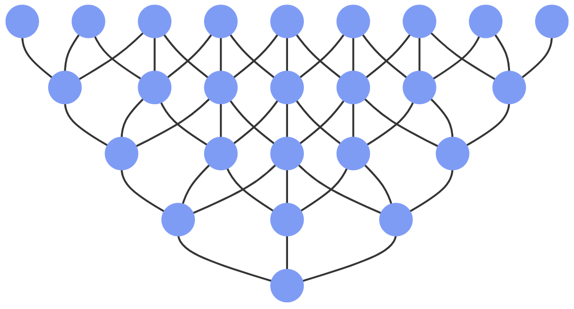
So what’s wrong with this code? The issue is that it’s doing the same work over and over again. Below is the call graph for fib(5). Notice how much repetition there is. This inefficiency only increases when computing larger numbers:

Memoization

Memoization to the rescue!

Memoization is a silly sounding word for “remembering results you’ve already found”. This next version of the code uses a Python dict to remember previous results. It doesn’t bother recalculating something that’s already in the cache:

cache = {}
count = 0
def fib2(n):
    global cache, count
    if n not in cache:
        count += 1
        cache[n] = 1 if n <= 2 else fib2(n-1) + fib2(n-2)
    return cache[n]
print(fib2(n), count)

fib2(40) calculates the correct result in only 40 steps (compared to over 200 million earlier).

We just did dynamic programming. Well, maybe. I personally believe this meets the definition of dynamic programming, but others say top-down recursive implementations don’t count.

In the next step, I’ll convert to a bottom-up approach that everyone agrees is dynamic programming.

Flipping the problem upside down

fib2() still uses a top-down recursive approach. In most instances of dynamic programming, it’s possible to solve the problem bottom up by anticipating what subproblems will need to be solved. In the case of Fibonacci, this is quite easy. To calculate the 40th number in the sequence, you need to first calculate the first 39.

This version of the code drops the recursive approach and uses a list instead of a dict to remember the calculated results:

def fib3(n):
    fibs = []
    for i in range(n):
        if i < 2:
            fibs.append(1)
        else:
            fibs.append(fibs[i-1] + fibs[i-2])
    return fibs[-1]
print(fib3(n))

It’s easy to see that fib3(40) only does 40 iterations, so it’s as efficient as fib2(). It’s actually a bit better because it uses a more efficient data structure and dispenses with the deep call stack of the recursive implementation.

Finally, notice that the algorithm never looks back more than two steps, so you can get rid of the list altogether and just use two variables:

def fib4(n):
    a, b = 1, 1
    for _ in range(n-2):
        a, b = b, a+b
    return b
print(fib4(n))

This again requires only 40 iterations to compute fib4(40), but it has the added advantage of using only extra constant space.

What is dynamic programming?

Hopefully, the Fibonacci sequence example was intuitive for you and not at all scary. Now it’s time to introduce a little terminology so you can sound smart when you talk about it.

There are two necessary conditions for dynamic programming to work:

Your problem must have optimal substructure. This means that you can compute the correct result (e.g. the 40th Fibonacci number) just by computing subproblems (e.g. the 38th and 39th Fibonacci numbers). This is basically another way of saying that a recursive approach will work.
Your problem must have overlapping subproblems. This means that a simple recursive approach will do duplicate work. Think back to the call graph for the original fib() function. If the same subproblem shows up multiple times, you’ll benefit from using dynamic programming.

Here are the steps to apply dynamic programming:

Formulate a recursive solution.
Use memoization to avoid recalculating subproblems.
Use a bottom-up approach to avoid recursion.
Optimize space efficiency by forgetting results you no longer need.

You’re allowed to skip steps if you already know how to get there. For example, many of you probably thought of the simple iterative approach to Fibonacci immediately.

Seam carving

In the rest of this post, I’ll walk through another dynamic programming example. This algorithm is called “seam carving”, or sometimes “content aware image resizing”.

The problem is as follows. You’re given a grid, and each cell in the grid has an associated (nonnegative) cost. Your job is to find a minimum cost path from any cell in the top row to any cell in the bottom row. Each step in the path has three choices: southwest, south, or southeast. The total cost of the path is the sum of the costs of each cell in the path.

That description might be hard to follow, so I’ll show you a small example:

The task is to find a path from the top row to the bottom row that’s minimal cost:

Starting with the 1, there are two options of where to go: straight down or diagonally down and to the right. The cheapest path is the latter. Total cost: 1 + 5 = 6.
Starting with the 2, all three options are available next. The cheapest is going diagonally down and to the right. Total cost: 2 + 3 = 5.
Starting with the 4, the cheapest path is straight down. 4 + 3 = 7.

For now, I don’t care about the full path, just its total cost. In this simple example, the cost of the best path is 5.

Now I’ll build a dynamic programming solution, step by step.

Step 1: Formulate a recursive solution

There’s a straightforward recursive solution to find the best path given a starting cell:

grid = [[4, 5, 4, 7, 8, 1, 6, 3, 5, 3],
        [9, 5, 4, 1, 3, 4, 3, 1, 9, 9],
        [6, 3, 3, 5, 9, 9, 8, 6, 3, 3],
        [3, 1, 7, 4, 2, 7, 3, 8, 7, 2],
        [6, 9, 5, 7, 9, 6, 3, 2, 3, 2]]
rows = len(grid)
cols = len(grid[0])

def mincost(r, c):
    # Bottom row is the base case.
    if r == rows-1:
        return grid[r][c]

    return grid[r][c] + min(
        # Minimum of SW, S, and SE neighbors, but skip out-of-bounds ones.
        mincost(r+1, cp) for cp in (c-1, c, c+1) if 0 <= cp < cols
    )

overall_min = min(mincost(0, i) for i in range(cols))

Below is that solution in action. Just press “Start” and watch the (slow) magic. There’s an artificial delay of 40ms for each function call so you can follow the progress:

A little blue number in a cell represents the total cost of the best path starting at that cell. If you’re patient enough to watch the whole thing (about 40 seconds), you’ll see the best possible path cost highlighted in green.

Notice how much duplicate work is happening. The overlapping subproblems are computed again and again.

As with the Fibonacci example, I’ve counted the function calls to see just how much dynamic programming can help. This simple top-down recursive implementation uses 1,012 function calls to compute the best path in a 10×5 grid.

Step 2: Use memoization

This version of the code simply stores the minimum cost for each cell as it’s computed:

cache = {}
def mincost2(r, c):
    if r == rows-1:
        return grid[r][c]

    if (r, c) not in cache:
        cache[r, c] = grid[r][c] + min(
            mincost2(r+1, cp) for cp in (c-1, c, c+1) if 0 <= cp < cols
        )
    
    return cache[r, c]

I only changed a couple lines, but watch the dramatic improvement. (There’s still that 40ms delay so you can see things happen.)

There are 50 cells in the grid, and this solution uses exactly 50 function calls. (Compare to 1,012 for the non-memoized version.)

Another exponential function has turned linear with memoization!

Step 3: Use a bottom-up approach

If you watch the previous example, you’ll see that the grid is filled in diagonally, revealing that the top-down approach is still in effect. In this next iteration, I’ll flip the problem upside down and compute costs from the bottom up instead.

The following code computes the minimum cost for each cell in order, starting at the bottom left and ending at the top right:

# Start with an empty grid.
mcs = [[None] * cols for _ in range(rows)]

# Populate the bottom row.
mcs[-1] = grid[-1][:]

# For each remaining row, working our way up:
for r in range(rows-2, -1, -1):
    # Find the minimum using the row below.
    mcs[r] = [
        grid[r][c] + min(
            mcs[r+1][cp] for cp in (c-1, c, c+1) if 0 <= cp < cols
        )
        for c in range(cols)
    ]
overall_min = min(mcs[0])

Step 4: Optimize space efficiency

Once a row has been filled with minimum costs, there’s no reason to keep any of the rows below it. In this version, just one row of values is stored, so mcs becomes a 1-dimension array instead of 2-dimensional:

# Start with bottom row costs.
mcs = grid[rows-1][:]

# For subsequent rows, working our way up:
for r in range(rows-2, -1, -1):
    # Find the minimum using the row below.
    mcs = [
        grid[r][c] + min(
            mcs[cp] for cp in (c-1, c, c+1) if 0 <= cp < cols
        )
        for c in range(cols)
    ]
overall_min = min(mcs)

Reading the whole path

I said earlier that this example is called “seam carving”. Seam carving is a way to reduce the dimensions of an image in a way that keeps as much information as possible.

To do this, seam carving finds and removes a minimum cost path from top to bottom (or side to side) of an image, where the cost of each pixel is something like its gradient magnitude. Edges in the image have the highest gradient magnitude, so they will be preserved as much as possible.

Removing the pixels along a vertical path reduces the width of the image by one pixel. This process is then repeated to remove more columns (or rows, using horizontal paths).

Up to this point, I’ve only cared about the cost of the minimum path, but now I actually need the path itself. To get that, I’ll go back to keeping the full grid around. Once the starting cell is known, it’s easy to find the full path. At each step, just look down one row and see which neighbor has the lowest minimum cost. That’s the next step in the path.

This final example puts it all together and computes the minimum path efficiently:

Trade those random numbers in for pixel gradients, and you have seam carving! Seam carving is pretty neat, so I’ll leave you with this video that shows it in action: